If you are reading this post chances are you are a relative of mine or you want to get insights about neural nets.
Only one week since beginning of the -unique in its kind- Jeremy Howard and Rachel Thomas’ Fastai international course 1v2. The amount of information and code flowing is already overwhelming, and it’s just the beginning.
I know that if I wait for the dust to settle and everything to be tidy in my head I will contribute and post when I am 90 year old. So, my plan, if I think an idea can help anyone that is just a small step behind me I will post it.
Fast.ai deep learning first lesson uses the famous Kaggle competition dataset “dogs vs. cats” to show binary classification with pretrained convnets. Even if you think “I have done that already” I advise you to watch the video in some months from now when it becomes public. Because I also “have done that already” but the approaches, tips, and opinions Jeremy Howard gives as well as the tools are… well, just as intended, both cutting edge and fully usable.
One of the most impressive of those tools is the “learning rate finder”. This tool implements the techniques described in the paper Cyclical Learning Rates for Training Neural Networks by Leslie N. Smith.
Implications of this are quite revolutionary. Anyone that has ever tried to make a neural net “learn” knows that it is difficult. Usual parameter search methods don’t work well and are slow. Finding proper learning rate, the most important of those parameters is both time consuming and difficult. That was, until last week.
To find the optimal range of values for learning rate the technique proposed is to increase the learning rate from a very small value until the loss starts decreasing, moment in which learning rate across batches is ploted. This is how this tool looks like in action:
LEARNING RATE ACROSS BATCHES (batch size = 64)
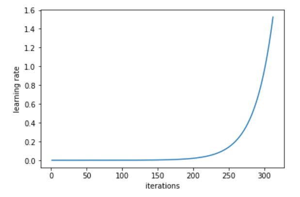
Note that 1 iteration in previous plot refers to 1 minibatch iteration of SGD
LOSS VS. LEARNING RATE (batch size = 64)
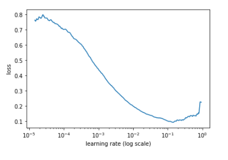
The plot shows Loss vs. Learning rate for the dataset. Now it is easy to choose an optimal range for learning rate before the curve flattens.
So simple -once discovered- that surprises how revolutionary this is. It has the potential to save a huge amount of hours and computational resources as soon as it becomes widespread practice. Aditionally to realizing this I also thought about how insightful it would be to use the tool to visualize the famous relationship between learning rate and batch size.
For the ones unaware, general rule is “bigger batch size bigger learning rate”. This is just logical because bigger batch size means more confidence in the direction of your “descent” of the error surface while the smaller a batch size is the closer you are to “stochastic” descent (batch size 1). Small steps can also work but the direction of each individual “steps” is more… well, more stochastic.
So… let’s see how it looks like. In this case it is true that a picture is worth one thousand words:
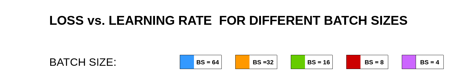
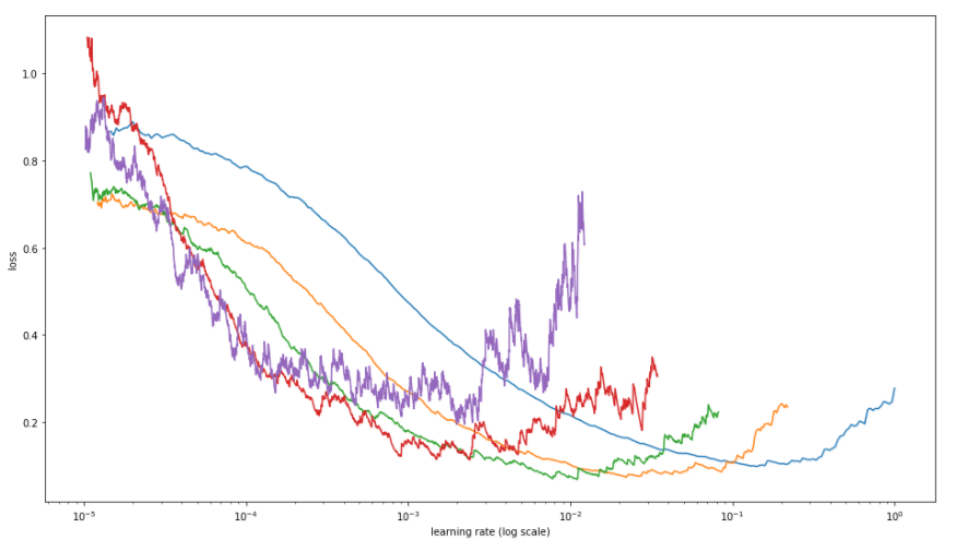
There you have it, the relationship between learning rate error plotted using batches from 64 to 4 for the “cats vs. dogs” dataset.
As expected bigger batch size shows bigger optimal learning rate, but the picture gives a more subtle and complete information. I find it interesting to see how those curves relate to each other, also worth noting how noise of the relationship increases as batch size gets smaller.
So, that was it, my first post and hopefully not the last one, hope you enjoyed it!